Assessing tree species diversity in forest ecosystems: A new approach

Introduction

The concept of biodiversity has evolved rapidly during the past decades. It is widely accepted that biodiversity can be divided into three spheres: genetic diversity (within-species diversity), species diversity (number of species), and ecosystem diversity (diversity of communities) (Harper and Hawksworth, 1995; Wilson and Peter, 1988). Typically, the focus is on species diversity. The relationship between biodiversity and ecosystem functioning and productivity has received increasing attention within the scientific community during the past decades (McNaughton, 1994; Hooper et al., 2005). The continuous loss of protophyte biodiversity due to human activities, invasion of alien species and climate change have led to negative effects on ecosystem functions and stability (Naeem et al., 1994; Hooper et al., 2012; Flombaum et al., 2016). Biodiversity research has therefore developed to become an important part of conservation biology and functional ecology (Ma, 2013, 2016). Species diversity is a crucial concept of biodiversity and is intuitively simple yet conceptually complex. A quantitative assessment of species diversity is thus essential for effective biodiversity conservation and management (Magurran, 2004).

Measures of species diversity usually include two components: richness and evenness. Richness represents the total number of species within a given area, while evenness measures how similar species are in their abundances (Hurlbert, 1971; Magurran, 2004). Species richness and evenness are two independent criteria that may differ in their responses to local habitat factors (Fisher et al., 1943; Preston, 1948; MacArthur, 1957; Ma, 2005). Recent empirical studies have demonstrated that the relationship between species richness and evenness appears to be weaker than expected (Wilsey et al., 2005; Soininen et al., 2012). These two diversity components may vary independently and could be influenced by different ecological processes. For example, in a forest ecosystem with highly diversified, extreme weather or natural disasters may cause large-scale species extinction, which reduces species richness, but may increase the evenness of species distribution. A number of studies have shown that species evenness could also exhibit strong impacts on ecosystem productivity and other functions as richness does (Wilsey and Potvin, 2000; Wittebolle et al., 2009; Zhang et al., 2012). For example, Wilsey and Potvin (2000) have shown that plant biomass increased linearly with increasing species evenness in Canadian grasslands. It appears logical therefore, that species evenness and richness should both be considered to gain a deeper understanding of the effects of different species diversity patterns (Weiher and Keddy, 1999; Crowder et al., 2012).

Various indices have been proposed to capture information about the diversity of a plant community (Margalef, 1958; Hill, 1973; Purvis and Hector, 2000; Wilsey and Potvin, 2000; Magurran, 2004; Hui et al., 2011; Chao et al., 2013). The principal objective of a diversity index is to obtain a quantitative estimate of biological variability that can be used to compare biological entities in space or time. Species diversity indices can be divided into simple and composite indices (Morris et al., 2014). The most common simple index is species richness. However, this index always ignores or under-emphasizes abundance information (Wilsey et al., 2005). Composite indices, which combine species richness and evenness into a single value, are widely used in ecology. Such indices have benefits of being simple to calculate and having a long history of application. However, most of them prefer to express the information of only one component between richness and evenness, and sacrifice the information of another component, such as the Shannon–Weaver (H′) (Shannon and Weaver, 1949) and Simpson index (D) (Simpson, 1949), which are the most common indices used for describing species diversity in forest communities (Swindel et al., 1984; Cao and Zhang, 1997; Rubio et al., 2011; Hakkenberg et al., 2016).

The requirement, discussed earlier that species evenness should be calculated independently of richness, is a disadvantage of both these two composite indices (Morris et al., 2014). Combining richness and evenness into a single value may lead to counter-intuitive species diversity results, because such composite indices rely on unequal weight between species richness and evenness. For example, a species-rich community with low evenness could have a lower Shannon–Weaver index value than another community with low richness and higher evenness (Duelli and Obrist, 2003). The Simpson index is ambiguous since the same index value may be obtained for communities with different species frequencies (Buckland et al., 2005). Other evenness indices, which are derived from the Shannon–Weaver or Simpson index, have only limited application predictively because they mathematically correlate with these indices.

An additional major drawback of a composite index is the ambiguity of its definition (Hurlbert, 1971). For example, the Shannon–Weaver index can be interpreted as a measure of the uncertainty in the identity of an individual randomly selected from a community, where a higher degree of uncertainty implies greater diversity (Shannon, 1948). This index seems to be one with no direct biological interpretation. The Simpson index is a probability which also does not have a straight-forward, let alone ecologically meaningful interpretation (Tuomisto, 2010, 2012). Despite a long history of use, doubt appears to still exist regarding both the understanding and interpretation of these indices (Stirling and Wilsey, 2001; Hill et al., 2003). It has been suggested that understanding of diversity lay not the form of the numbers (e.g., probabilities), but in the ecological meaning of the variation in the abundance values which is the basis for calculating such indices (Tuomisto, 2010). From this perspective, it is needed to propose a D_RE with meaningful biological interpretation.

Accordingly, this study takes the tree species in the forest as an example and introduce a new diversity measure (called D_RE), which should have the following characteristics: (1) It can independently express the tree species richness and evenness in the community; (2) It has the characteristics of classical and can express the general law of community diversity. (3) It is sensitive to the changes of tree species richness and evenness, and can analyses the contribution of tree species richness and evenness to community diversity.

Materials and methods

Simulated data

In order to evaluate the effectiveness of the new tree species D_RE, a series of simulated communities were established with the number of tree species ranging from 3 to 100, and their relative frequency ranging from 0.8 to 0.002 (more details are presented in Table 1). These simulated communities are assumed to be representative, i.e., each community included both the dominated and rare species. The simulated datasets were then used to calculate the values of different tree species diversity indices.

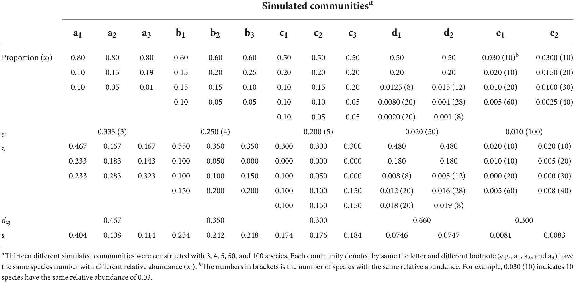
Table 1. Frequency distributions of different simulated communities with the same absolute discrepancy (d_xy).

Field data

The effectiveness of different species diversity indices was also compared using observed field data. The field data used in this study were collected in 15 plots of different forest types distributed along an environment gradient (Table 2). The vegetation type in the Jiaohe forest region is a temperate coniferous and broad-leaved mixed forest, and the main tree species are Fraxinus mandshurica, Pinus koraiensis, Juglans mandshurica, Carpinus cordata, and Abies holophylla. The Jiulongshan forest is a warm-temperate broad-leaved deciduous forest with artificially planted Platycladus orientalis as the main tree species, and also includes naturally regenerated Quercus variabilis, Broussonetia papyrifera, Ailanthus altissima, Prunus davidiana, and Spina gleditsiae. The Xiaolongshan forest region is situated at the warm temperate-subtropical transitional zone. In this region, the natural forest type is a pine-oak mixed forest composed of Quercus aliena var. acuteserrata and Quercus liaotungensis. The main tree species include Quercus aliena var. acuteserrata, Quercus liaotungensis, Pinus armandii, Pinus tabulaeformis, Populus davidiana, Rhus verniciflua, and Kalopanax septemlobus. The artificial forest type includes mainly Pinus armandii and Pinus tabulaeformis plantations, which are mixed with naturally regenerated Quercus acuteserrata, Tilia paucicostata, Crataegus kansuensis, and Pyrus xerophila. The Liping forest region belongs to subtropical humid evergreen broad-leaved natural forest type, where the main tree species are Castanopsis tibetana, Castanopsis fabri, Cyclobalanopsis glauca, Castanopsis carlesii, Castanopsis eyrei, Castanopsis kweichouensis, Schima superba, Daphniphyllum oldhamii, Liquidambar formosana, and Quercus acutissima. The Jianfengling forest region is a tropical mountane rain forest, and the mian tree species in this area are Cryptocarya chinensis, Gironniera subaequalis, Mallotus hookeriana, Nephelium lappaceum, Livistona carinus, and Schima superba.

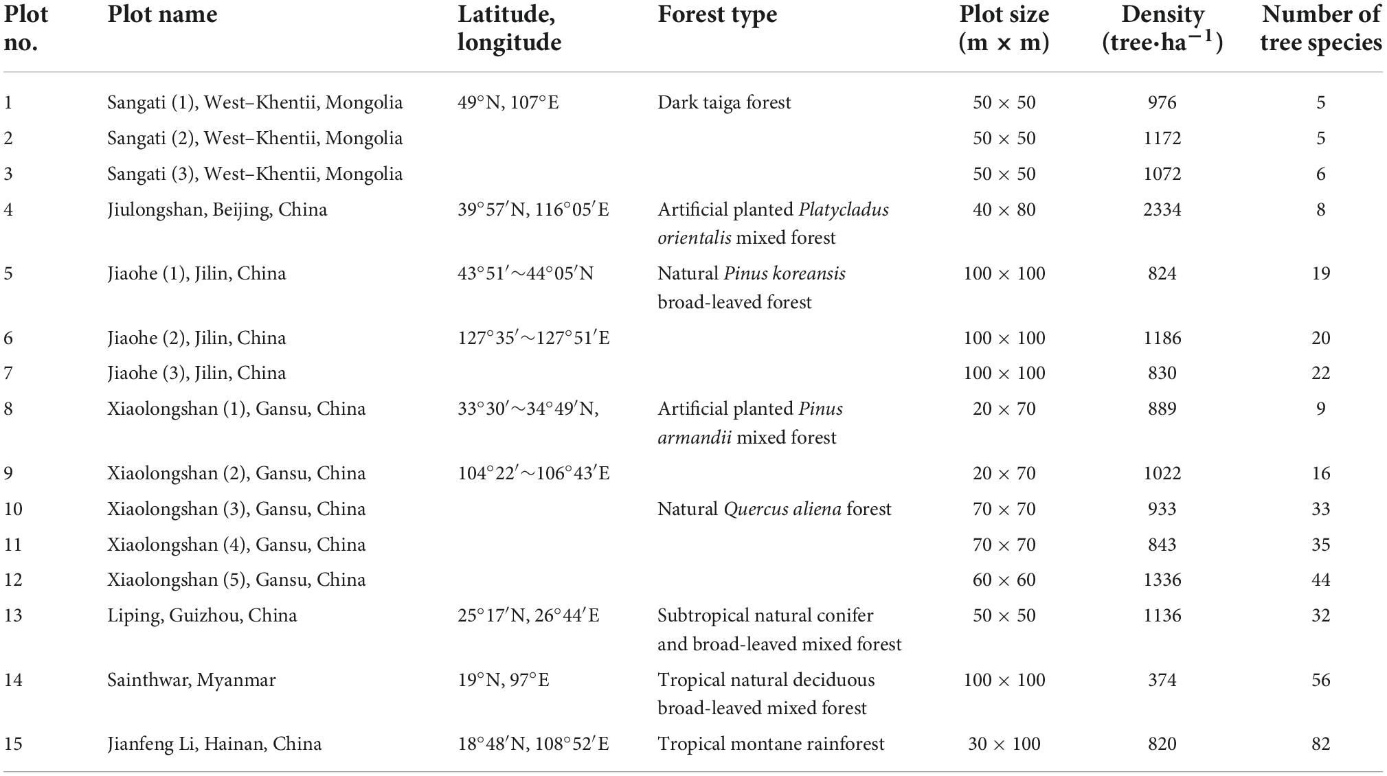
Table 2. Details of field plots belonging to different forest types locating in different climate zones.

The Sangati research area in Northern Mongolia represents old growth “dark” taiga forest and is situated near the KhoninNuga ecological research station in the West–Khentii province, near the Eruu River and bordering on the strictly protected area of Khan Khentii. The main tree species in this area are Abies sibirica, Larix gmelinii, Picea obovata, and Pinus sibirica.

The Sainthwar research forest, situated near the village Sainthwar in the Paunglaung watershed of Myanmar, has been classified as a tropical natural deciduous broad-leaved mixed forest. Altogether 30 tree species are found in this forest, including Pterocarpus macrocarpus, Dalbergia oliveri, Mitragyna rotundifolia, Adina cordifolia, Albizia odoratissima, Dalbergia cultrate, Melanorrhoea usitata, Tectona grandis, and Baccaurea sapida.

Indices and measurement of species diversity

Species evenness reflects the relationship between the number of individuals of each species and the total number of all individuals in a community. It refers to the uniformity of the relative abundance of different tree species (biomass, coverage, or other indicators) in the community. Here we give a definition of the absolute uniform community, that is, all species in the community have the same relative abundance, thus the evenness can be expressed by comparing the difference between relative abundance of the number of tree species of the investigated community and absolute uniform community with the same species. The smaller the difference between the observed community species distribution and the community with completely uniform species distribution, the greater the evenness is. Gregorius (1974) proposed a measure of absolute discrepancy (d_xy) for measuring the allelic differentiation between two relative frequency distributions:

where x_i is the relative frequency of hereditary form i in the community X; y_i is the relative frequency of hereditary form i in the community Y; k denotes the quantity of hereditary forms; it is easy to see that.

Eq. (1) has been widely used to compare the difference between two populations, to identify whether two field plots are from the same totality, or to measure the difference between two ecosystems (Hui and Albert, 2004). In this way, d_xy is the sum of the dissimilarity between the observed and the uniform community, and has the following important characteristics: (1) d_xy is a non-negative real number; (2) the distance is symmetric, i.e., d_xy = d_yx; and (3) if the genetic structures of community X and Y are completely consistent, d_xy is equal to 0, i.e., the two communities have the same allelic frequencies. The maximum value of d_xy is 1.

When the absolute discrepancy formula [Eq. (1)] is used for measuring a forest community, the corresponding variables are defined in the following: x_i is relative frequency of tree species i in community X, and y_i is the expected relative frequency in absolute uniform community Y which all tree species abundances are homogenous (same frequencies of different species, i.e., y_i = 1/k, where k is the number of species), and z_i is the absolute difference between x_i and y_i, i.e.,(x_i − y_i). Table 1 presented species frequency distributions of a series of simulated communities that consist of 3, 4, 5, 50, and 100 tree species.

As d_xy is independent of the distribution of x_i – y_i, the same value of d_xy may be obtained for different species distributions as shown in Table 1. For example, there have same three tree species in communities a₁, a₂, and a₃ and they have the same d_xy = 0.467, but they are different in species frequency distributions. The same situation occured in other simulated communities b, c, d, and e, and in these communities also have the same tree species with different distribution frequency. This non-determinacy of the measure of absolute discrepancy reduces its reliability and stringency. At the same time, we also found that the standard deviation(s) of species frequency between communities with the same d_xy is different from Table 1 (see the last row in Table 1), which suggests that we can characterize the difference between communities through d_xy and its standard deviation of tree species frequency in each community group. Therefore, to overcome this deficiency of the absolute discrepancy, use the following equation to modify d_xy through adding the standard deviation (s) of the distribution of the differences x_i – y_i.

Where x_i is the distribution frequency of tree species in the community X; y_i is the distribution frequency of tree species i in the absolute uniform community Y; s is standard deviation of the distribution of the differences x_i – y_i Eq. (2) thus measures the non-evenness of any community attributes including tree species, tree diameter (or height) and structural variables. Conversely, evenness (SE) can be calculated using the following equation:

where the value of SE ranges between 0 and 1. The greater the value of SE, the greater the tree species evenness is, and vice versa. In addition, when all tree species in an observed community share the same relative abundance as the uniform community does, the tree species evenness reaches a maximum value of 1.

How to combine tree species richness and evenness independently? A simple addition or combination of k and SE will inevitably increase the weight of richness on diversity and reduce that of evenness, because the latter only assumes values between 0 and 1, while the former may assume any great number. Hence, for an effective combination of these two criteria, tree species richness must be normalized to the assumed values between 0 and 1. Logarithmic transforms can be used to eliminate the problem of large orders of magnitude of community tree species number. Here, the specific method is to logarithmically transform tree species number and normalize its values between 0 and 1. The reason for logarithmic transformation is that logarithmic function is a monotonically increasing function in its range of definition, which is consistent with the relationship between tree species richness and species number. Logarithmic transformation not only can reduce the absolute value of tree species number (reducing the variable scale and relatively stabilizing the numerical fluctuation), but also improve the sensitivity to small numbers and keep the relative size relation between tree species numbers. This can be presented as:

The purpose of dividing k by 2 in formula 4 is that K_log should be 0 when only two species exist (k = 2). This is because that the necessary condition for tree species diversity studies is at least two species existing in a community to represent biodiversity (k ≥ 2). Thus, tree species richness assumes a minimum value when the community has only two species.

After the elimination of magnitude difference in tree species numbers, species richness is normalized by comparing k_log with the logarithm of the possible largest species number in a biotic community (K_logmax). This normalization can be achieved by using the following expression:

The logarithm transformation of k greatly reduces the range of k_logmax, and the number of tree species in forest communities is assumed to be far less than 1,000, thus k_logmax will be less than 3 for forest communities. Previous researches showed, in species-rich forest communities (e.g., tropical rainforest), the number of tree species in a given sample is commonly less than 2000 (Gadow and Hui, 2007; Chuyong et al., 2011). When k reaches 2000 (k_max = 2000), for example, the tree species in the forest community is extraordinarily abundant, $k_{lo{g}_{max}}=\log \left(\frac{2000}{2}\right)=3$. Eq. (5) can be simplified as:

where SR represents the normalized species richness (k). The constraint of Eq. (6) for forest communities is 2 ≤ k ≤ 2000, thus the range of SR is 0 ≤ SR ≤ 1.

After unifying the numerical ranges of species richness and evenness (both are between [0 and 1]), their normalized dimensionless values can be directly mathematically combined, i.e., diversity (D_RE) can be expressed by using the mean values of richness (SR) and evenness (SE) as biodiversity is a unification of species richness and evenness. Both the arithmetical mean (addition relationship, Eq. (7)) and geometric mean [multiplication relationship, Eq. (8)] of richness (SR) and evenness (SE) can be used to express biodiversity (D_RE).

D_RE [Eq. (7) or Eq. (8)] has the following characteristics: (1) the value of D_RE ranges between 0 and 1, i.e., between minimum and maximum biodiversity, respectively; (2) in the case of equal evenness, the greater species richness, the higher the diversity; (3) in the case of equal richness, the greater the evenness, the greater the diversity; and (4) species richness and evenness can be calculated independently.

For comparative purpose, the Shannon–Weaver index (Shannon and Weaver, 1949) [H′, Eq. (9)], Simpson (Simpson, 1949) [D, Eq. (10)] and the Hill Numbers or the effective number (1973) [^qD, Eq. (11)] were also calculated for each data set at the same time.

where s is the number of species and p_i is the proportion of the sample belonging to the ith species.

where p_i is the proportion of the sample belonging to the ith species. As biodiversity increases, the Simpson index decreases. Therefore, D′ = 1-D is used in this study.

where s is the number of species, p_i is the proportion of the sample belonging to the ith species and q is called the “order” of the diversity measure. Species richness is a diversity index of order 0, Shannon entropy is a diversity index of order one, and all Simpson measures are diversity indices of order two. The order q determines a diversity measure‘s sensitivity to rare or common species (Hill, 1973; Keylock, 2005; Jost, 2007; Chao et al., 2010, 2014).

Sensitivity analysis

A series of simulations were performed to evaluate the relative sensitivity of different species diversity and evenness indices to species richness and evenness. For species richness, we created a series of uniform communities, in which the number of species decreased from 50 to 3, and the relative change rate (RCR) of different diversity indices were compared. For species evenness, we created a series of communities where the number of rare species increased from 1 to 7, and then the RCR of different evenness indices were also compared. The used species diversity indices were H′, D′ and the new constructed richness index SR [Eq. (6)]. The used species evenness indices were the Pielou evenness index [calculated as J′ = H′/ln(k), where H′ is the Shannon–Weaver index, and k is the species number], the Simpson evenness index [calculated as D_E = (1/D)/k, where D is the Simpson diversity index and k is the species number], and the new evenness index SE [Eq. (3)]. The RCR was defined as RCR = [(A_j-A_i)/A_i] × 100%, where A_i is the value of index in A_i community, and A_j is the value of index in A_j community. The value of RCR is high when an index varies widely for a set of simulated communities.

Results

Using diversity index to measure the tree species diversity of simulated communities

Table 3 shows the values of the ^qD, H′, D′, d_xy, s, SE, SR, D_{R + E}andD_R×E indices of the thirteen simulated communities. The new constructed tree species diversity index (D_{R + E}andD_R×E) exhibited variation similar to that of the traditional diversity indices (^qD, H′, and D′), where all of these five indices increased with increasing tree species number (k) or richness (SR). In the case of the same k or SR, different tree species evenness values (SE) could result in different diversities, and the diversity increased with increasing SE. Through calculating tree species evenness (SE) and richness (SR) independently, the new diversity index (D_{R + E}orD_R×E) could directly indicate the cause for the increase in tree species diversity. The reason that D_RE expressed biodiversity effectively could be mainly due to the modification of the discrepancy index (d_xy) for measuring the difference between two relative frequency distributions. The modified discrepancy index (d’_xy) distinguished between different communities with the same discrepancy (d_xy) but different frequency distributions (x_i), through adding the standard deviation (s) of the distribution of the differences x_i – y_i. This modification helped to express the species evenness more precisely.

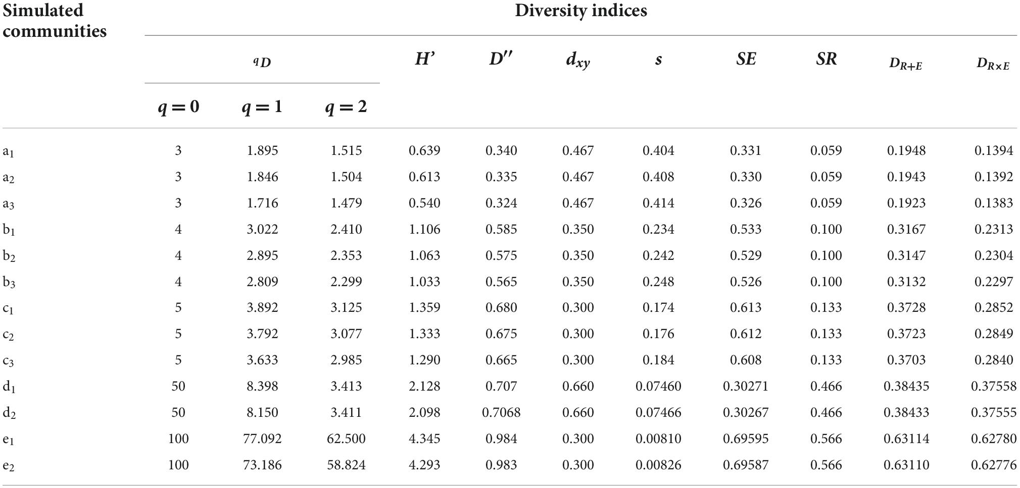
Table 3. Compared the value of different diversity indices using the simulated datasets in Table 1.

Using D_RE to measure the species diversity of natural forests in different climate zones

As shown in Table 4, the new index D_RE may be used to describe the general variation of species diversity in natural forests, similarly to the diversity indices of ^qD, H′, and D′. The biodiversity in the tropical forest (plot 15; D_R+E = 0.573; D_R×E = 0.574) was the highest, followed by that in the tropical deciduous broad-leaved forest (plot 14; D_R+E = 0.494; D_R×E = 0.494), the subtropical conifer and broad-leaved mixed forest (plot 13; D_R+E = 0.487; D_R×E = 0.480), the pine-oak mixed forest in the warm temperate-subtropical transitional zone (plot 10–12; D_R+E = 0.428; D_R×E = 0.428), the Pinus koreansis broad-leaved forest in the temperate zone (plot 5–7; D_R+E = 0.426; D_R×E = 0.416), and the taiga forest in the cold temperate zone (plot 1–3; D_R+E = 0.265; D_R×E = 0.234). For the same climate zone, D_{R + E}≥D_R×E (SE and SR ∈ R⁺).

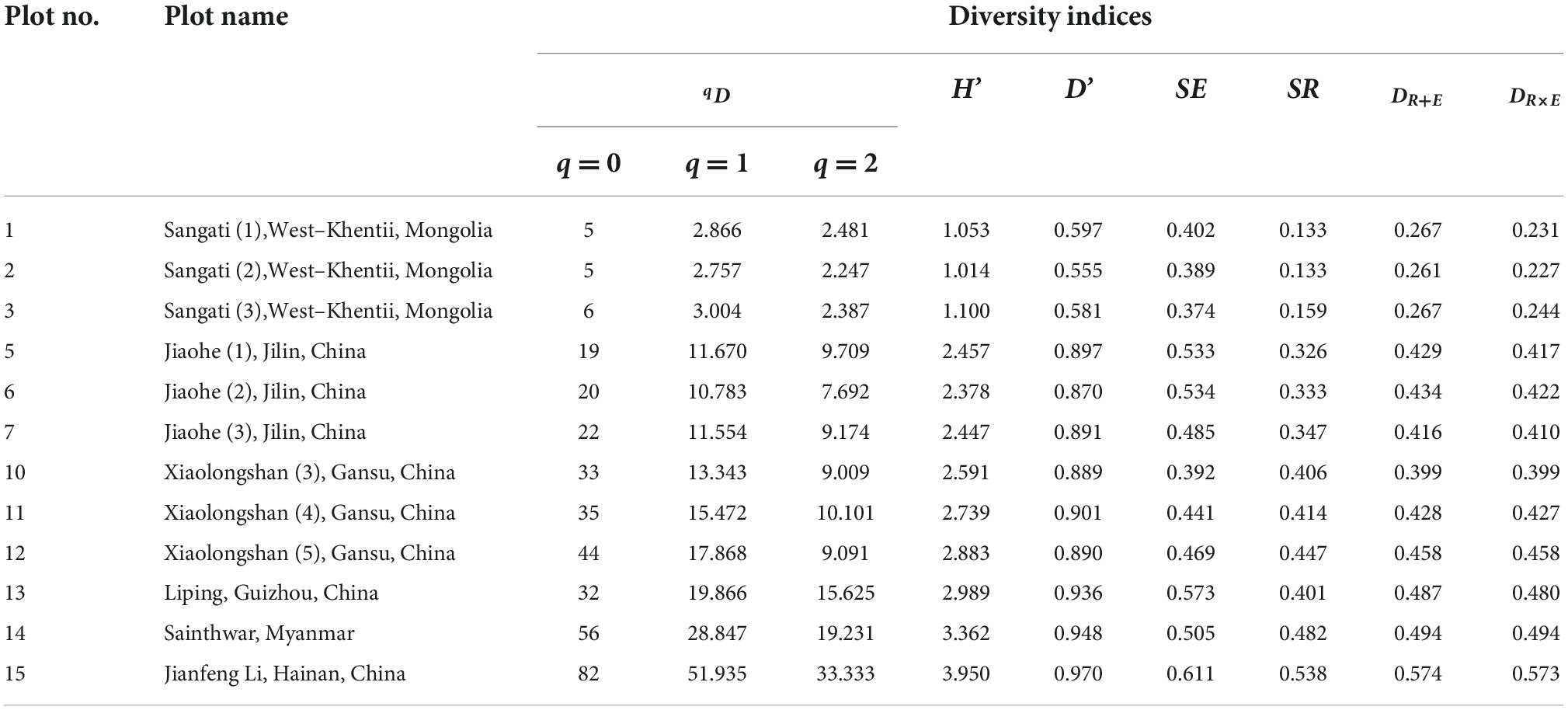
Table 4. Tree species diversity of natural forests locating in different climate zones.

It should be noted that, although the tree species number in the Liping forest region located in subtropical zone was lower than that in the Xiaolongshan forest region located in the warm temperate-subtropical transitional zone, all of these five diversity indices indicated that the tree species diversity of the former forest region was higher than the latter (Table 4). According to Eqs (7, 8), the higher diversity in the Liping forest region was mainly due to the greater tree species evenness. In addition, within the same climatic zone, the rank order of different plots were not the same for different indices (Table 4). This phenomenon might be attributed to the relative importance of evenness and richness in the different diversity indices.

Using D_RE to measure the tree species diversity of artificially mixed forests

Table 5 shows the tree species diversity of three artificial mixed forests. In the Jiulongshan forest region, located in the northern warm temperate zone, Platycladus orientalis accounted for 87% of the trees in the artificial P. orientalis mixed forest, while the remaining 13% trees were composed of seven naturally regenerated tree species. All the four diversity indices (^qD, H′, D′,D_{R + E}andD_R×E) indicated that the species diversity in this forest region was lower than that in the Xiaolongshan forest region, which is situated at the warm temperate-subtropical transitional zone.

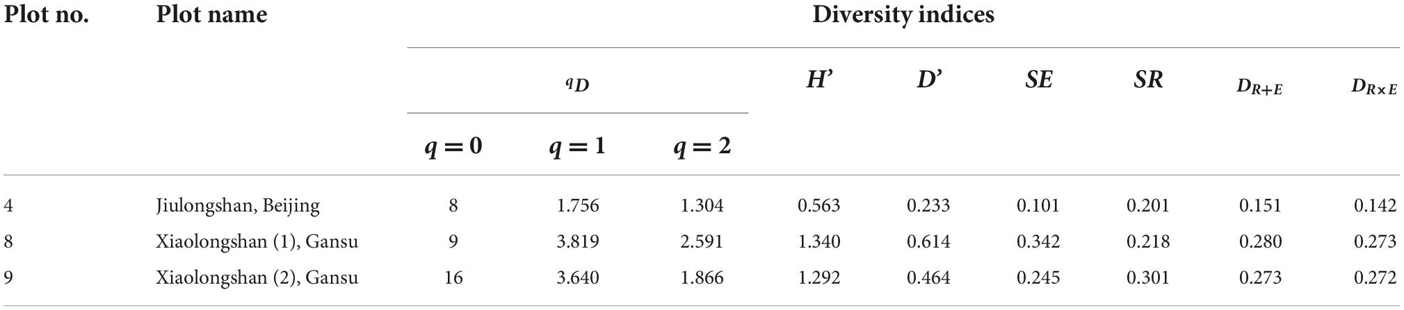
Table 5. Tree species diversity of different artificial mixed forests locating in different climate zones.

It should be noted that the species diversity of the two plots (plot 8, 9; Table 2) in the Xiaolongshan forest region expressed by the new diversity index (D_R+E) was rather different from that expressed by D_R×E and the diversity indices (^qD, H′, and D′). As shown in Figure 1, plot 8 was composed of Pinus tabulaeformis, Pinus armandii and seven other naturally regenerated tree species, the species frequency of which were 57.5, 21.3, and 21.2%, respectively. In contrast, plot 9 was mainly composed of P. armandii, which accounted for 72.8% of trees, while the remaining trees were represented by fifteen naturally regenerated tree species with relatively low frequencies. The calculated D_R+E indicated that the species diversity of plot 9 with sixteen tree species was higher than that of plot 8 with nine tree species [D_R+E(16) = 0.349 > D_{R+E ⁽⁹⁾} = 0.335]. However, ^qD, H′, D′, and D_R×E exhibited a higher species diversity in plot 8 with 9 tree species. It can be seen from Table 5 that D_RE and Hill number were completely consistent when expressing species evenness [SE₍₈₎ = 0.342 > SE₍₁₆₎ = 0.245], while the “order” of q was 2 and the Hill number was 2.591 and 1.866, respectively. When the “order” of the Hill number of q was 0, the species richness was 8 and 16, respectively. The SR of sample plot 8 and sample plot 9 was 0.218 and 0.301, respectively, the trend of richness of two indexes also have the same result. However, the new diversity index of D_RE exhibited a higher species diversity in plot 9 with 16 tree species, this may be due to the new index assignment higher weight to richness.

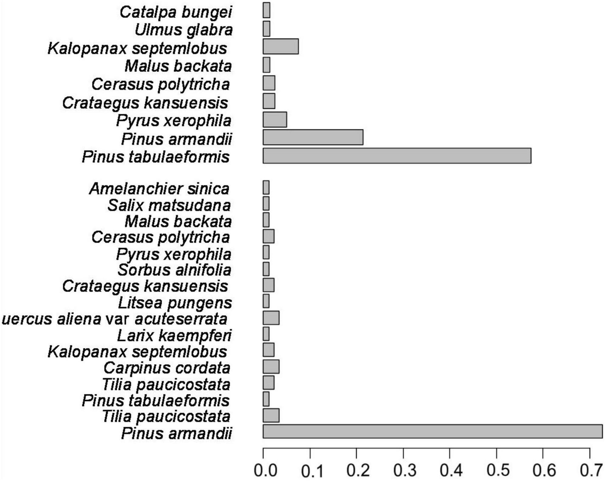
Figure 1. Distribution of species relative frequency (x_i) of plantations in Xiaolongshan mountain.

Sensitivity analysis of different tree species diversity indices based on a set of simulated communities

Figure 2 illustrates the RCR of three species richness and evenness indices with changing compositions of the simulated communities. Different indices show different sensitivities to the variation of the number of species or rare species, and the new richness (SR) and evenness (SE) indices had superior statistical behavior relative to the other two richness and evenness indices, respectively. In a homogenous community, as the number of species decreases from 50 to 3, the value of SR decreases more sharply than the Shannon–Wiener and Simpson diversity indices (Figure 2A). Similarly, with the increase of the rare species in a simulated community from 2 to 7, the new evenness index (SE) also exhibited the highest RCR among the three evenness indices (Figure 2B).

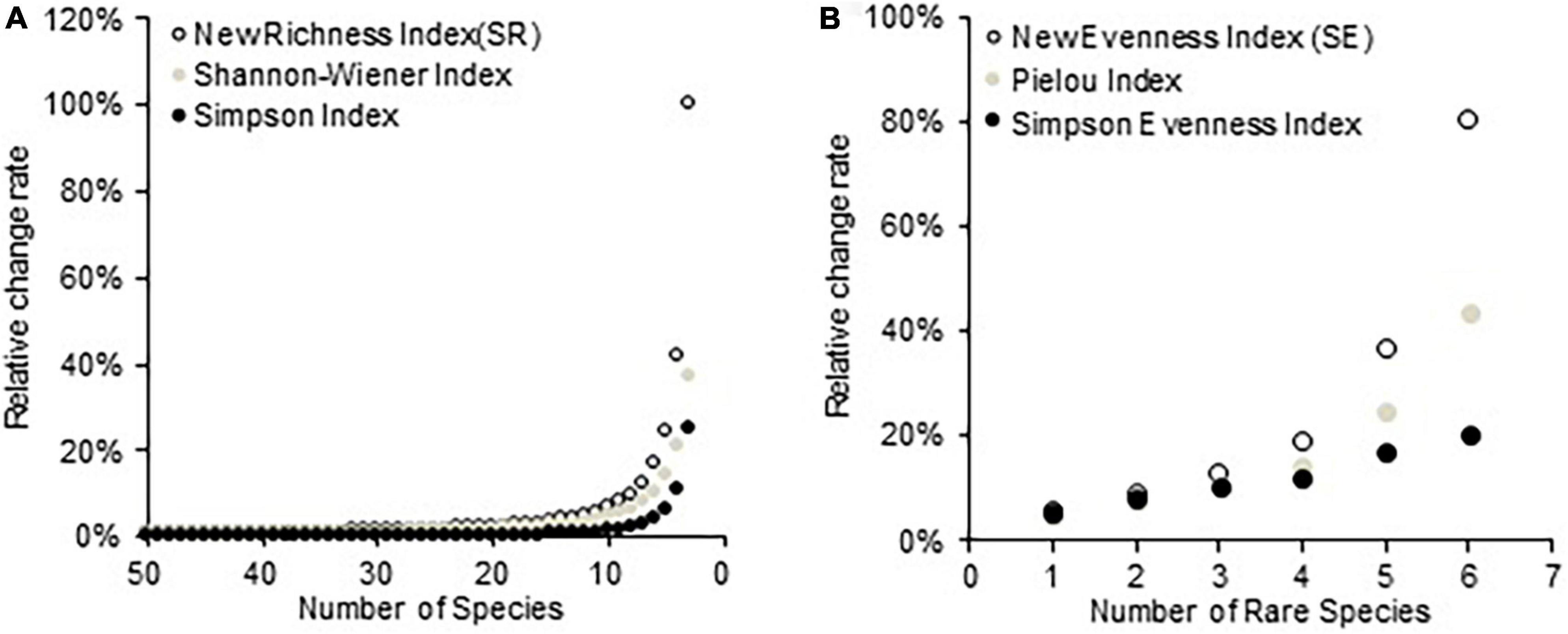
Figure 2. (A) Relative change rates of three diversity indices to the variation of species number in a series of simulated communities and (B) relative change rates of three evenness indices to the variation of rare species number in a series of simulated communities.

Discussion

As demonstrated in the results section, the new diversity index is sensitive to different patterns of species diversity in different climatic zones. This result indicates that the climate and disturbance account for a large proportion of the variation of biodiversity (Gaston, 2000; Hawkins et al., 2003). The main practical advantage of the proposed D_RE measure over other indices is that species richness and evenness are treated independently, and equal weight is given to richness and evenness. The results of field observed data demonstrated that these characteristics were important for an unambiguous and accurate assessment of biodiversity. When we use the traditional indices (H′ and D′) to assess the diversity in the artificial mixed forest communities (Table 5 and Figure 1), which are dominated by a single planted species and mixed with a few naturally regenerated tree species, such abundance distribution result in a drastic drop of evenness and hence yields low values of traditional diversity indices, in spite of comparatively higher species richness. In contrast, the proposed D_RE measure describes richness and evenness independently, and reveals diversity patterns more accurately in these rather uneven communities, without any loss of information. The Simpson and Shannon–Wiener indices are calculated exclusively from abundance values, it is thus difficult to assess the contribution of richness to the variation in D′ and H′ (Yue et al., 2007; Strong, 2016). Therefore, Whittaker (1972) argued that the Simpson index is primarily a measure of dominance, especially of the first 2–3 species, whereas the Shannon–Weaver index is more strongly affected by species in the middle of the rank sequence of species. Thus, the two indices measure different aspects of species diversity. As a result, the actual relationships among species relative abundances are distorted. Such distortion could easily lead to a misinterpretation of diversity (Jost, 2007).

Hill numbers or the effective number of species are increasingly used to quantify species diversity of an assemblage and recently extended to phylogenetic diversity and functional diversity. The Hill numbers are a parametric family of diversity indexes differing among themselves only by the parameter q that determines sensitivity to species relative abundance. It provides the number of equally abundant species that are needed to give the same value of a diversity measures (Chao et al., 2010, 2014). Compare the diversity calculation results of simulated sample plots (Table 4) and the investigated natural forest sample plots (Table 5), it is found that the trend of species richness and evenness of new diversity D_RE (SR and SE) with Hill numbers (q = 0 and q = 2) are almost identical. There only few species evenness of sample plots were differences. The main reason may be that SE expresses evenness by comparing the difference of the tree species distribution frequency between investigated community and absolute uniform community, while the Hill number is abundance-based species diversity of the investigated community and it is believed as the best choice to quantify true diversity. Any evenness index should measure the equality of abundances in the community and maximum evenness occurs when all species are equally abundant (Alatalo, 1981). The more the relative abundances of species differ, the smaller is the evenness value. The modified absolute discrepancy formula [Eq. (3)] can measure dissimilarities between an observed community and a uniform community through comparing the species relative abundances. Our evenness index was found to be most easily interpreted: the more similar the observed and the uniform community are, the more even is the observed community. This interpretation reflects the concept of species evenness.

On the other hand, the assessment of richness in the new index is directly related to the number of species. The use of logarithmic transformation in the new species richness index (SR) can effectively describe the real change of diversity when adding a new species to different diversity communities. For instance, as to a species-poor community, adding a new species would make a big contribution to the species diversity. However, for a species-rich community, adding a new species would make only a slight contribution to the species diversity. In general, theoretical ecologists suggested that a satisfactory index of species evenness must assume values between 0 and 1 (Stirling and Wilsey, 2001; Camargo, 2008). Both the new evenness and species richness indexes are a normalized expression to assume values between 0 and 1. By doing this, the normalized dimensionless richness and evenness indexes can be easily combined to express diversity based on the ecological meaning and significance. The general statement “species diversity consists of two independent components, evenness and richness” logically lead us to use the mean values of evenness and richness as a combination method to express diversity; hence, this also produces a new diversity index that have normalized dimensionless values between 0 and 1. Both the arithmetical mean (addition relationship, D_R+E) and geometric mean (multiplication relationship, D_R×E) of richness and evenness were applied to yield diversity for our simulated and field data. We found that both D_R+E and D_R×E increased as the climate zone ranging from warm temperate to subtropical transitional zone, but for the same forest community, D_{R + E} ≥ D_R×E (Tables 4, 5). One special situation is that the calculated D_R+E for the two plots (plot 8, 9; Table 2) in the Xiaolongshan forest region showed discrepant values (D_R+E = 0.280 and 0.273, respectively), while D_R×E yielded two similar values (D_R+E = 0.273 and 0.272) for these two stands with different species richness (9 species for plot 8 and 16 species for plot 9). This is primarily because the geometric mean is biased toward the estimation of the population mean and its value is always less than the arithmetic mean unless all numbers in the dataset are the same producing equal arithmetic mean and geometric mean. The arithmetic mean is easy to calculate and understand, however, the arithmetic mean is more affected by extreme values than the geometric mean. Therefore, we suggest that the new biodiversity index D_R×E is more universally applicable, while D_R+E may be limited to small sample data subject to lognormal distribution (Parkhurst, 1998).

According to our analysis, the new species index (D_RE) has at least two characteristics of other diversity indexes. Firstly, it independently express diversity from the aspects of evenness (RE) and richness of species (SR) and compared with other traditional diversity index it is more sensitive to the abundance changes of rare species. This feature is better than traditional diversity (e g., H′ and D′) and allows us to analyze the causes of diversity changes, which better reflects the concept that diversity is composed of species evenness and richness. Secondly the new index provides minimum value 0 and maximum values 1 and the greater the value, the higher the diversity. The interpretation of the results is more intuitive and meaningful. However, it also has some limitations of new metric that it doesn‘t obey the replication principle like other traditional diversity (e.g., H′ and D′). In this respect, the Hill number has more obvious advantages and it can provide more information. In addition, this study only analyzed the tree species diversity in the forest community as an example, and whether it can be used for analysis of other systems or whether it can be further extended to phylogenetic diversity and functional diversity needs further in-depth study.

Conclusion

This study presents a new approach to measure tree species diversity in forest ecosystem. According to our analysis, the new tree species diversity index (D_RE) independently expresses the richness and the evenness of tree species aboundance distribution in the community. These two aspects are combined to express the tree species diversity of the community and its value ranges between 0 and 1. Like other classical D_RE (^qD,H′, and D′), the new index can express the general law that the tree species diversity of the community increases with the increase of tree species. A remarkable feature of the new index is that it is sensitive to changes in the richness and evenness of tree species in the community, and can analyze the contribution of tree species richness and evenness to tree species diversity, which has important practical significance for understanding the structure and carrying out community monitoring and protection.

Data availability statement

The original contributions presented in this study are included in the article/supplementary material, further inquiries can be directed to the corresponding author.

Author contributions

ZZ, GH, and YH provided the idea. ZZ and GH calculated and analyzed the data. AY and GZ supported the data investigate. All authors contributed to the manuscript.

Funding

The authors gratefully acknowledge the National Natural Science Foundation of China (Funding number: 32171780) and the Basic Research Fund of CAF (Funding number: CAFYBB2020ZB002-1).

Conflict of interest

The authors declare that the research was conducted in the absence of any commercial or financial relationships that could be construed as a potential conflict of interest.

Publisher’s note

All claims expressed in this article are solely those of the authors and do not necessarily represent those of their affiliated organizations, or those of the publisher, the editors and the reviewers. Any product that may be evaluated in this article, or claim that may be made by its manufacturer, is not guaranteed or endorsed by the publisher.

References

Alatalo, R. V. (1981). Problem in the measurement of evenness in ecology. Oikos 37, 199–204. doi: 10.2307/3544465
Buckland, S. T., Magurran, A. E., Green, R. E., and Fewster, R. M. (2005). Monitoring change in biodiversity through composite indices. Philos. Trans. R. Soc. B 360, 243–254. doi: 10.1098/rstb.2004.1589
Camargo, J. A. (2008). Revisiting the relation between species diversity and information theory. Acta Biotheoretica 56, 275–283. doi: 10.1007/s10441-008-9053-x
Cao, M., and Zhang, J. (1997). Tree species diversity of tropical forest vegetation in Xishuangbanna, SW China. Biodivers. Conserv. 6, 995–1006. doi: 10.1023/A:1018367630923
Chao, A., Chiu, C.-H., and Jost, L. (2010). Phylogenetic diversity measures based on Hill numbers. Philos. Trans. R. Soc. B 365, 3599–3609. doi: 10.1098/rstb.2010.0272
Chao, A., Chiu, C. H., and Jost, L. (2014). Unifying species diversity, phylogenetic diversity, functional diversity, and related similarity and differentiation measures through hill numbers. Annu. Rev. Ecol. Evol. Syst. 45, 297–324. doi: 10.1146/annurev-ecolsys-120213-091540
Chao, A., Wang, Y. T., and Jost, L. (2013). Entropy and the species accumulation curve: a novel entropy estimator via discovery rates of new species. Methods Ecol. Evol. 4, 1091–1100. doi: 10.1111/2041-210X.12108
Chuyong, G. B., Kenfack, D., Harms, K. E., Thomas, D. W., Condit, R., and Comita, L. S. (2011). Habitat specificity and diversity of tree species in an African wet tropical forest. Plant Ecol. 212, 1363–1374. doi: 10.1007/s11258-011-9912-4
Crowder, D. W., Northfield, T. D., Gomulkiewicz, R., and Snyder, W. E. (2012). Conserving and promoting evenness: organic farming and fire-based wildland management as case studies. Ecology 93, 2001–2007. doi: 10.1890/12-0110.1
Duelli, P., and Obrist, M. K. (2003). Biodiversity indicators: the choice of values and measures. Agric. Ecosyst. Environ. 98, 87–98. doi: 10.1016/S0167-8809(03)00072-0
Fisher, R. A., Corbet, A. S., and Williams, C. B. (1943). The relation between the number of species and the number of individuals in a random sample of an animal population. J. Animal Ecol. 12, 42–58. doi: 10.2307/1411
Flombaum, P., Yahdjian, L., and Sala, O. E. (2016). Global change drivers of ecosystem functioning modulated by natural variability and saturating responses. Glob. Change Biol. 23, 503–511. doi: 10.1111/gcb.13441
Gadow, V. K., and Hui, G. Y. (2007). Can the tree species-area relationship be derived from prior knowledge of the tree species richness. For. Study 46, 13–22.
Gregorius, H. R. (1974). Zur Konzeption der genetischen abstandsmessung: Genetischer abstand zwischen populationen. Silvae Genetica 23, 22–27.
Hakkenberg, C. R., Song, C., Peet, R. K., and White, P. S. (2016). Forest structure as a predictor of tree species diversity in the North Carolina Piedmont. J. Veg. Sci. 27, 1151–1163. doi: 10.1111/jvs.12451
Harper, J. L., and Hawksworth, D. L. (1995). “Preface,” in Biodiversity: Measurement and Estimation, ed. D. L. Hawksworth (London, UK: Chapman & Hall), 5–6.
Hawkins, B. A., Field, R., Cornell, V. H., Currie, D. J., Guégan, J. F., Kaufman, D. M., et al. (2003). Energy, water, and broad-scale geographic patterns of species richness. Ecology 84, 3105–3117. doi: 10.1890/03-8006
Hill, M. O. (1973). Diversity and evenness: a unifying notation and its consequences. Ecology 54, 427–432. doi: 10.2307/1934352
Hill, T. C. J., Walsh, K. A., Harris, J. A., and Moffett, B. F. (2003). Using ecological diversity measures with bacterial communities. FEMS Microbiol. Ecol. 43, 1–11. doi: 10.1111/j.1574-6941.2003.tb01040.x
Hooper, D. U., Adair, E. C., Cardinale, B. J., Byrnes, J. E. K., Hungate, B. A., Matulich, K. L., et al. (2012). A global synthesis reveals biodiversity loss as a major driver of ecosystem change. Nature 486, 105–108. doi: 10.1038/nature11118
Hooper, D. U., Chapin, F. S. I. I. I., Ewel, J. J., Hector, A., Inchausti, P., Lavorel, S., et al. (2005). Effects of biodiversity on ecosystem functioning: a consensus of current knowledge. Ecol. Monogr. 75, 3–35. doi: 10.1890/04-0922
Hui, G. Y., and Albert, M. (2004). Stichprobensimulationen zur Schätzung nachbarschaftsbezogener Strukturparameter in Waldbeständen. Allgemeine Forst-u. Jagdzeitung 175, 199–209.
Hui, G. Y., Zhao, X. H., Zhao, Z. H., and Gadow, V. K. (2011). Evaluating tree species spatial diversity based on neighborhood relationships. For. Sci. 57, 292–300.
Hurlbert, S. H. (1971). The nonconcept of species diversity: a critique and alternative parameters. Ecology 52, 577–586. doi: 10.2307/1934145
Jost, L. (2007). Partitioning diversity into independent alpha and beta components. Ecology 88, 2427–2439. doi: 10.1890/06-1736.1
Keylock, C. (2005). Simpson diversity and the Shannon-Wiener index as special cases of a generalized entropy. Oikos 109, 203–207. doi: 10.1111/j.0030-1299.2005.13735.x
Ma, K. P. (2013). Studies on biodiversity and ecosystem function via manipulation experiments. Biodivers. Sci. 21, 247–248. doi: 10.3724/SP.J.1003.2013.02132
Ma, K. P. (2016). Hot topics for biodiversity science. Biodivers. Sci. 24, 1–2. doi: 10.17520/biods.2016029
Ma, M. (2005). Species richness vs evenness: independent relationship and different responses to edaphic factors. Oikos 111, 192–198. doi: 10.1111/j.0030-1299.2005.13049.x
MacArthur, R. H. (1957). On the relative abundance of bird species. Proc. Natl. Acad. Sci.U.S.A. 43, 293–295. doi: 10.1073/pnas.43.3.293
McNaughton, S. J. (1994). “Biodiversity and function of grazing ecosystems,” in Biodiversity and Ecosystem Function, eds E. D. Schulze and H. A. Mooney (Berlin Heidelberg, DE: Springer), 361–383. doi: 10.1007/978-3-642-58001-7_17
Morris, E. K., Caruso, T., Buscot, F., Fischer, M., Hancock, C., Maier, T. S., et al. (2014). Choosing and using diversity indices: insights for ecological applications from the German Biodiversity Exploratories. Ecol. Evol. 4, 3514–3524. doi: 10.1002/ece3.1155
Naeem, S., Thompson, L. J., Lawler, S. P., Lawton, J. H., and Woodfin, R. M. (1994). Declining biodiversity can alter the performance of ecosystem. Nature 368, 734–737. doi: 10.1038/368734a0
Parkhurst, D. F. (1998). Peer reviewed: arithmetic versus geometric means for environmental concentration data. Environ. Sci. Technol. 32:92A–98A. doi: 10.1021/es9834069
Preston, F. W. (1948). The commonness, and rarity, of species. Ecology 29, 254–283. doi: 10.2307/1930989
Purvis, A., and Hector, A. (2000). Getting the measure of biodiversity. Nature 405, 212–219. doi: 10.1038/35012221
Rubio, A., Gavián, R. G., Montes, F., Gutiérrez-Girón, A., Díaz-Pines, E., and Mezquida, E. T. (2011). Biodiversity measures applied to stand-level management: Can they really be useful? Ecol. Indicator 11, 545–556. doi: 10.1016/j.ecolind.2010.07.011
Shannon, C. E. (1948). A mathematical theory of communication. Bell. Syst. Technical. J. 27, 379–423. doi: 10.1002/j.1538-7305.1948.tb01338.x
Shannon, C. E., and Weaver, W. (1949). The Mathematical Theory of Communication. Urbana, IL: University of Illinois Press.
Soininen, J., Passy, S., and Hillebrand, H. (2012). The relationship between species richness and evenness: a meta-analysis of studies across aquatic ecosystems. Oecologia 169, 803–809. doi: 10.1007/s00442-011-2236-1
Stirling, G., and Wilsey, B. (2001). Empirical relationships between species richness, evenness, and proportional diversity. Am. Naturalist 158, 286–299. doi: 10.1086/321317
Strong, W. L. (2016). Biased richness and evenness relationships within Shannon-Wiener index values. Ecol. Indicator 67, 703–713. doi: 10.1016/j.ecolind.2016.03.043
Swindel, B. F., Conde, L. F., and Smith, J. E. (1984). Species diversity: concept, measurement, and response to clear cutting and site-preparation. For. Ecol. Manag. 8, 11–22. doi: 10.1016/0378-1127(84)90082-3
Tuomisto, H. (2010). A consistent terminology for quantifying species diversity? Yes, it does exist. Oecologia 164, 853–860. doi: 10.1007/s00442-010-1812-0
Tuomisto, H. (2012). An updated consumer’s guide to evenness and related indices. Oikos 121, 1203–1218. doi: 10.1111/j.1600-0706.2011.19897.x
Weiher, E., and Keddy, P. A. (1999). Relative abundance and evenness patterns along diversity and biomass gradients. Oikos 87, 355–361. doi: 10.2307/3546751
Whittaker, R. H. (1972). Evolution and measurement of species diversity. Taxon 21, 213–251. doi: 10.2307/1218190
Wilsey, B. J., Chalcraft, D. R., Bowles, C. M., and Willig, M. R. (2005). Relationships among indices suggest that richness is an incomplete surrogate for grassland biodiversity. Ecology 86, 1178–1184. doi: 10.1890/04-0394
Wilsey, B. J., and Potvin, C. (2000). Biodiversity and ecosystem functioning: importance of species evenness in an old field. Ecology 81, 887–892. doi: 10.1890/0012-9658(2000)081[0887:BAEFIO]2.0.CO;2
Wilson, E. O., and Peter, F. M. (1988). “Snout moths: Unraveling the taxonomic diversity of a speciose group in the Neotropics,” in Biodiversity, eds E. O. Wilson and F. M. Peter (Washington, DC: National Academies press), 228–240.
Wittebolle, L., Marzorati, M., Clement, L., Balloi, A., Daffonchio, D., Heylen, K., et al. (2009). Initial community evenness favours functionality under selective stress. Nature 458, 623–626. doi: 10.1038/nature07840
Yue, T. X., Ma, S. N., Wu, S. X., and Zhan, J. Y. (2007). Comparative analyses of the scaling diversity index and its applicability. Int. J. Remote Sens. 28, 1611–1623. doi: 10.1080/01431160600887714
Keywords: absolute discrepancy, logarithmic transformation, normalization, relative abundances, species diversity, species evenness, species richness, uniform distribution
Citation: Zhao Z, Hui G, Yang A, Zhang G and Hu Y (2022) Assessing tree species diversity in forest ecosystems: A new approach. Front. Ecol. Evol. 10:971585. doi: 10.3389/fevo.2022.971585
Received: 21 June 2022; Accepted: 27 September 2022;
Published: 26 October 2022.
Edited by:
Christopher Swan, University of Maryland, Baltimore, United StatesReviewed by:
Paulo A. V. Borges, University of the Azores, PortugalWenhua Xiang, Central South University Forestry and Technology, China
Copyright © 2022 Zhao, Hui, Yang, Zhang and Hu. This is an open-access article distributed under the terms of the Creative Commons Attribution License (CC BY). The use, distribution or reproduction in other forums is permitted, provided the original author(s) and the copyright owner(s) are credited and that the original publication in this journal is cited, in accordance with accepted academic practice. No use, distribution or reproduction is permitted which does not comply with these terms.
*Correspondence: Yanbo Hu, hyanbo@caf.ac.cn